Absorption Systems#
Detecting and fitting absorption lines is the core mission of Astrocook. The software provides a tiered approach: fully automated pipelines for initial detection, and a dedicated System Inspector for detailed Voigt profile analysis and manual refinement.
1. Automated Detection Pipelines#
For most science cases, you should start with one of the automated pipelines in the Absorbers menu. These recipes scan the spectrum, identify features, and perform an initial fit.
Important
Normalization: All fitting recipes calculate absorption depth relative to the continuum. Astrocook uses the cont column (multiplied by telluric_model if present) as the reference.
If no continuum exists, the software assumes the flux
Fis already normalized (median \(\approx\) 1).To use an alternative continuum (e.g., a power-law
cont_pl), you must first copy it into the maincontcolumn using Edit > Apply Expression… (cont = cont_pl).
Note
This recipe requires Emission Redshift (\(z_{em}\)) and Resolution (\(R\)) to be defined. If missing, Astrocook will automatically prompt you to set them via the Set Properties dialog before proceeding.
Ly-alpha Forest#
If you are analyzing a high-redshift quasar (\(z > 2\)):
Ensure your Emission Redshift is set correctly.
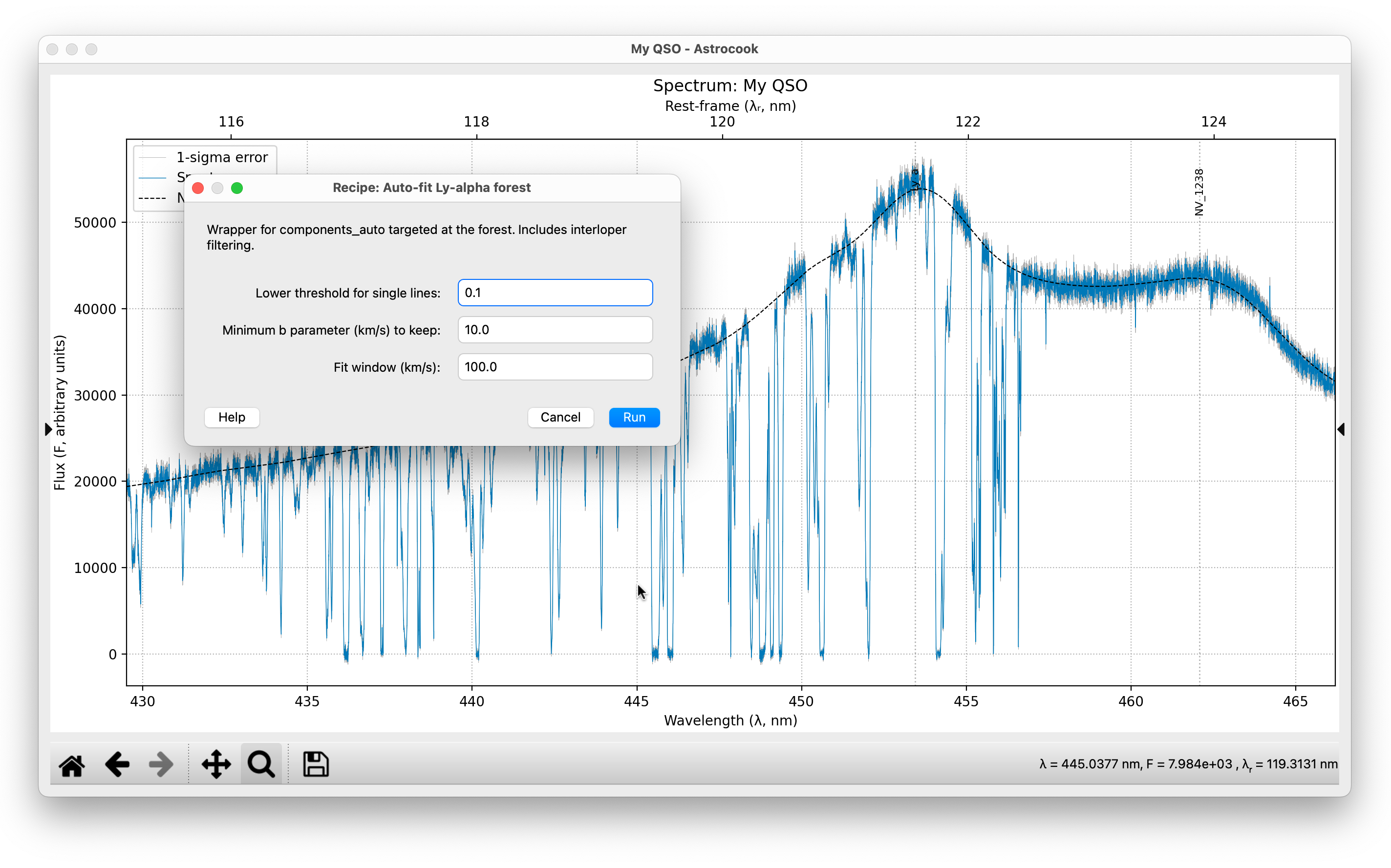
Go to Absorbers > Auto-fit Ly-alpha Forest….
Threshold: The default score (
0.1) is usually fine.Min b: The minimum Doppler parameter (e.g.,
10km/s) helps filter out noise spikes or unphysically narrow lines (interlopers).Click Run.
This pipeline focuses on the region between the Ly\(\beta\) and Ly\(\alpha\) emission lines.
Metal Doublets#
For finding distinct metal systems (CIV, SiIV, MgII) redward of the Ly\(\alpha\) emission:
Go to Absorbers > Auto-detect Doublets….
Multiplets: You can customize the list (e.g.,
CIV, SiIV, MgII).Click Run.
This recipe searches for pairs of lines with the correct velocity separation and optical depth ratios.
Note
This recipe requires Emission Redshift (\(z_{em}\)) and Resolution (\(R\)) to be defined. If missing, Astrocook will automatically prompt you to set them via the Set Properties dialog before proceeding.
General Detection#
For a more generic search (or if you are looking for specific ions):
Go to Absorbers > Identify Absorption Lines….
This generates a list of candidate regions but does not fit them immediately.
You can then visualize these regions by selecting
abs_idsin the Aux. Column dropdown of the Plot Controls.
Note
This recipe requires Emission Redshift (\(z_{em}\)) and Resolution (\(R\)) to be defined. If missing, Astrocook will automatically prompt you to set them via the Set Properties dialog before proceeding.
2. The System Inspector#
Once you have systems (either from a pipeline or added manually), the System Inspector is your cockpit for detailed analysis.
To open it: View > View System Inspector, or right-click over a component in the main window to display the context menu.
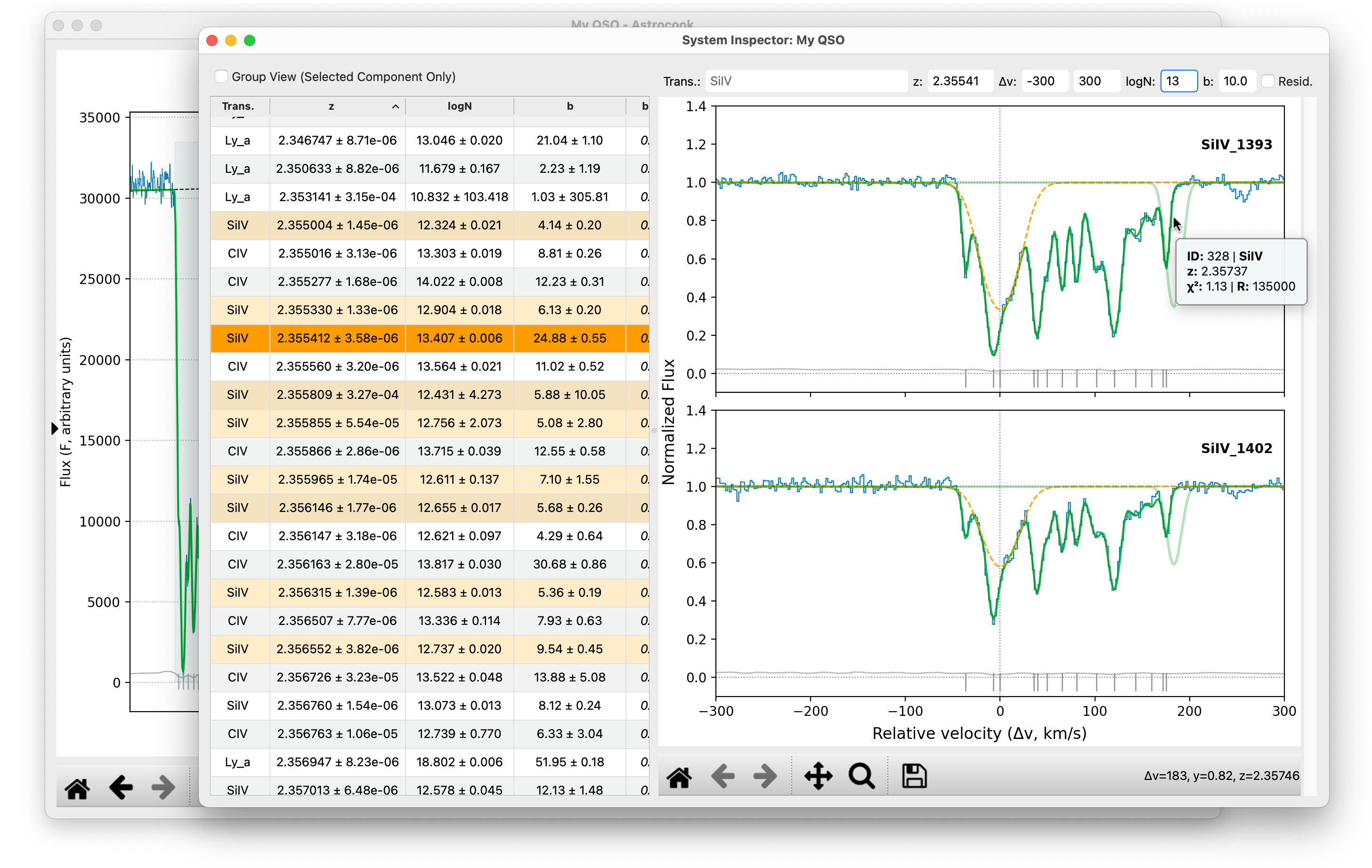
Left Panel: System List#
This table lists every component in the model.
Edit: Double-click any cell (
z,logN,b) to modify its value directly.Sort: Click any column header to sort the list (e.g., by Redshift or Series).
Tooltips: Hover over a row to see detailed fit statistics (\(\chi^2\)) and constraints status.
Resolution: Right-click a component to set a specific Resolution (\(R\)) for that line, overriding the global session default.
Group View: Check the box above the table to hide unrelated systems and show only the components physically linked to your selection.
Understanding Resolution Priority#
Astrocook handles instrumental resolution (\(R\)) flexibly to support both constant-resolution survey spectra and variable-resolution echelle data. The Voigt fitting engine and the velocity plots apply resolution convolution according to this strict hierarchy:
Component-Specific Resolution (Highest Priority): If you manually assign a resolution to a specific component (via the right-click menu in the System List), Astrocook will always use this value for that specific line, ignoring all other settings.
The
resolColumn: If your spectrum data contains aresolauxiliary column (visible in the Data Inspector), Astrocook will use the specific resolution value at the pixel where the absorption line is centered. This allows for accurate modeling of spectra where \(R\) changes with wavelength.Global Session Resolution (Fallback): If no component-specific override exists and no
resolcolumn is present, Astrocook falls back to the global scalar resolution set via Edit > Set Properties…. Note that setting a global resolution will automatically generate a flatresolcolumn across the entire spectrum.
Right Panel: Velocity Plot#
A zoomed-in view of the selected system in velocity space.
Navigation: The plot centers on the selected component. You can manually edit the Redshift (z) and Velocity Range (\(\pm v\)) using the text boxes above the plot.
Scroll: If a system has many transitions (e.g., Lyman series), use the scrollbar on the right to page through them.
Displayed Lines: The text box at the top shows which transitions are plotted (e.g.,
CIV, SiIV). You can type new ions here (comma-separated) to inspect other species at the same redshift.Test Component: The
logNandbboxes above the plot control the shape of the “ghost” profile attached to your mouse cursor, useful for visually estimating parameters before adding a component.Residuals: Check the Resid. box to show a residual plot below each transition panel.
3. Interactive Fitting & Editing#
The System Inspector allows you to modify the model dynamically.
Note
Just like in the main window, if the Zoom or Pan tools are active in the plot toolbar, you must hold Ctrl (or Cmd) while right-clicking to access the context menu.
Adding Components#
If the auto-finder missed a line:
In the Velocity Plot (right panel), Right-click on the background where the line should be.
The menu offers smart options based on the transition you clicked:
Add [Ion] (Single Line): Adds only the specific line under the cursor.
Add [Ion] (Standard): Adds the full standard multiplet (e.g., both members of the CIV doublet).
Add [List] (Subset): Adds exactly the set of transitions currently visible in the Inspector.
A new component is added and fitted immediately.
Note
This recipe requires Resolution (\(R\)) to be defined. If missing, Astrocook will automatically prompt you to set them via the Set Properties dialog before proceeding.
Tip
If you see multiple transitions in the menu (e.g., Add CIV-SiIV), this will add linked components for both ions at that redshift.
Constraints (Fix/Free)#
To fix a parameter during fitting:
Select the component(s) in the table.
Right-click to open the context menu.
Select Freeze ‘b’ (or
z,logN).The value will turn italic and the uncertainty display (\(\pm\)) will disappear, indicating it is fixed.
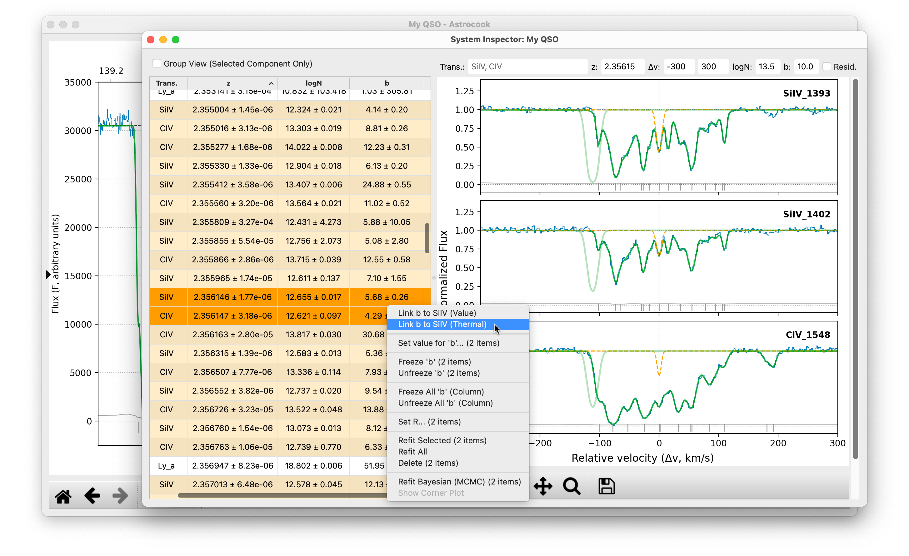
Parameter Linking#
Astrocook supports physical linking of parameters, which is essential for fitting doublets or multiphase systems.
Select two components in the table (hold
CtrlorCmd).Right-click on the parameter you want to link (e.g., the
zcolumn).Select Link z to [Other Component] (Value).
The value will turn bold, indicating it is dynamically calculated from the other component.
Doppler Parameter Linking: When linking the Doppler parameter b, you have two physical options:
Link (Value): Assumes the broadening is dominated by turbulence (or the ions have similar mass). The
bvalues are forced to be identical.Link (Thermal): Assumes the broadening is thermal. The
bvalue is scaled according to the atomic mass ratio of the two ions (\(b \propto m^{-1/2}\)).
Note
Astrocook also tracks a turbulent broadening parameter btur separately. It is available in the table but frozen (italic) by default. You can unfreeze it via the right-click menu if you need to model mixed thermal/turbulent broadening explicitly.
Refitting#
After manual edits, you often need to re-optimize the fit:
Refit Selected: Select one or more components in the table, right-click, and choose “Refit Selected”. This will optimize all highlighted lines (and their physical neighbors) in a batch process.
Refit All: Go to Absorbers > Refit All Systems… (in the main window) to re-optimize the entire spectrum, handling blends automatically.
Bayesian Fitting (Experimental)#
Astrocook v2 introduces a prototype Bayesian fitting engine, allowing you to rigorously explore parameter space using MCMC (emcee). This is particularly useful for analyzing highly blended systems or determining robust parameter uncertainties.
To run a Bayesian fit:
Select the component(s) you wish to fit in the System List.
Right-click to open the context menu and locate the Bayesian Fitting section.
Select Refit Bayesian (MCMC).
The sampling will run as a batch process, with progress tracked in the main window’s progress bar.
Visualizing Posteriors (Corner Plots) Once a Bayesian fit completes, Astrocook stores the posterior samples in the session metadata. You can visualize these directly:
Right-click a Bayesian-fitted component and select Show Corner Plot.
This opens a dedicated, scrollable window displaying the 1D histograms and 2D contours for all free parameters (\(z\), \(\log N\), \(b\)).
The plot title explicitly shows the median values along with their asymmetrical \(1\sigma\) uncertainties (e.g., \(14.500^{+0.123}_{-0.154}\)).
Auto-Refresh: You can leave the Corner Plot window open on a second monitor. As you click through different Bayesian-fitted systems in the table, or run new fits, the plot will automatically update to reflect the active system.
Note
While the corner plot displays the full asymmetric uncertainties, the main System List table simplifies these into a single, symmetric \(1\sigma\) equivalent (derived from the standard deviation of the samples) to maintain compatibility with legacy data structures.
Cleaning Results#
After running automated pipelines or performing manual fits, your model might contain artifacts such as noise spikes fitted as narrow lines, or continuum undulations fitted as broad, shallow features (“ghosts”).
Astrocook provides a dedicated tool to filter these out:
Go to Absorbers > Clean Negligible Components….
Min logN: Components weaker than this threshold (default
11.5) are removed.Min/Max b: Components narrower than
min_b(default3.0km/s) or broader thanmax_b(default80.0km/s) are flagged.Combined Check: By default (
True), broad lines are only removed if they are also very weak (logN < 13.0). This protects genuine broad features like DLA wings or OVI absorbers from being deleted.