Getting Started#
Welcome to Astrocook V2! This guide will walk you through the basics of the interface: loading data, exploring your spectra, and managing your analysis sessions.
1. Loading a Spectrum#
Let’s begin by loading some data. Astrocook supports various formats, including standard FITS files and its own archive formats (.acs, .acs2).
Launch Astrocook. You will be greeted by the welcome screen.
Go to the menu bar and select File > Open Session… (or press
Ctrl+O/Cmd+O).Select your spectrum file. You can select multiple files at once if you want to load several observations simultaneously.
Once loaded, the interface will come alive. The central area displays your spectrum, while two sidebars provide control over your data and visualization.
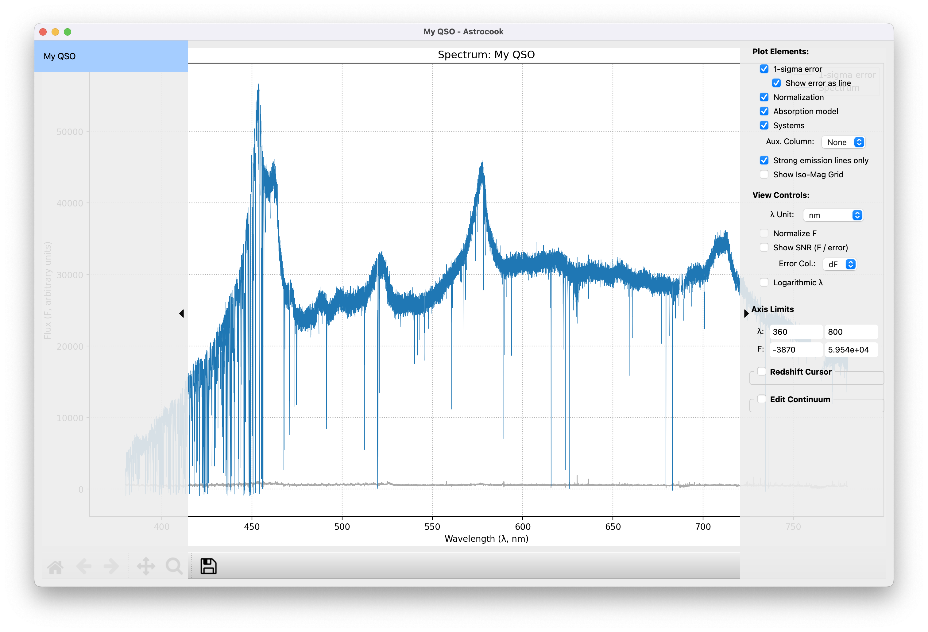
3. Customizing the View (Right Sidebar)#
Look to the right side of the window. This is the Plot Controls panel. Here you can tweak how the data is displayed without altering the data itself.
Toggles#
You can show or hide specific layers of the plot:
1-sigma error: Hides the grey error shading.
Show error as line: Instead of a shaded band, plots the error array (\(dy\)) as a separate line. Useful for inspecting noise structure in high-resolution spectra.
Normalization: Hides the continuum level (dashed black line).
Absorption model: Hides the Voigt profile fits (solid red line).
Systems: Hides the vertical tick marks indicating identified systems.
Aux. Column: Select an additional data column (e.g.,
abs_mask,running_std) to overlay on the plot.Strong emission lines: Shows markers for major emission lines (e.g., Ly-\(\alpha\), CIV).
Note
This requires defining the emission redshift first (see Setting Session Properties).
Show Iso-Mag Grid: Overlays curves of constant AB magnitude.
Note
This requires flux calibration (see Flux Calibration).
Axis Controls#
Units: You can switch the X-axis display between
nm,Angstrom, andmicronon the fly.Normalize F: Plots the flux relative to the continuum (showing \(f = F / F_\mathrm{cont}\)) (this control becomes active only when a
contcolumn is present).Show SNR: Plots the Signal-to-Noise Ratio instead of flux.
Error Col.: When showing SNR, you can select which column to use as the noise estimate (default is
dF).
Logarithmic \(\lambda\): Switches the X-axis to a logarithmic scale.
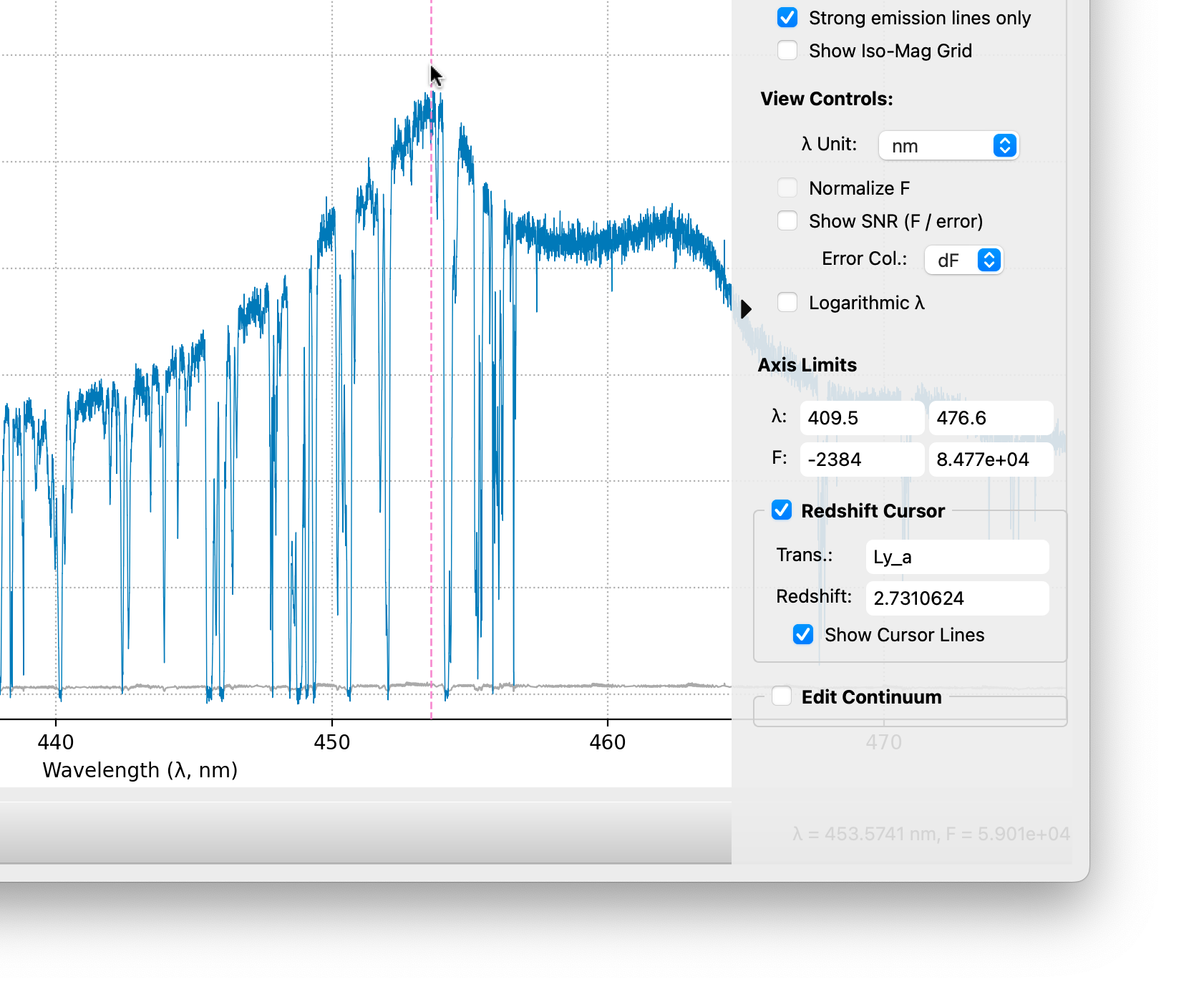
Axis Limits#
You can manually set the precise bounds of the plot view. Enter values for \(\lambda\) Min/Max and F Min/Max and press Enter to apply them. These boxes automatically update when you zoom or pan interactively.
The Redshift Cursor#
This is a handy tool for quick visual inspection.
In the Redshift Cursor section, enter a transition name (e.g.,
Ly_a,CIV,MgII) and a redshiftz.Check the Show Cursor Lines box.
Vertical dashed lines will appear on the plot indicating where that transition should be found. You can update the
zvalue to slide the cursor along the spectrum.
Interactive Setting: You can Right-click directly on the plot background to open a context menu. Select Set emission redshift to z=… to instantly update the session’s \(z_{em}\) based on the cursor’s current position.
Note
If the Zoom or Pan tools are active in the toolbar, the right-click shortcut is overridden. In this case, hold Ctrl (or Cmd on Mac) while right-clicking to access the context menu.
The Continuum Editor#
Located at the bottom of the sidebar, this panel allows you to interactively refine the continuum shape using spline knots. See the Interactive Manual Editing in the Continuum Fitting tutorial for a detailed guide on using the slider, spacing box, and editing tools.
4. Session Management (Left Sidebar)#
The panel on the left is your Session List. Each file you load becomes a “Session”.
Switching Sessions#
If you loaded multiple spectra, click on their names in this list to switch the main view instantly.
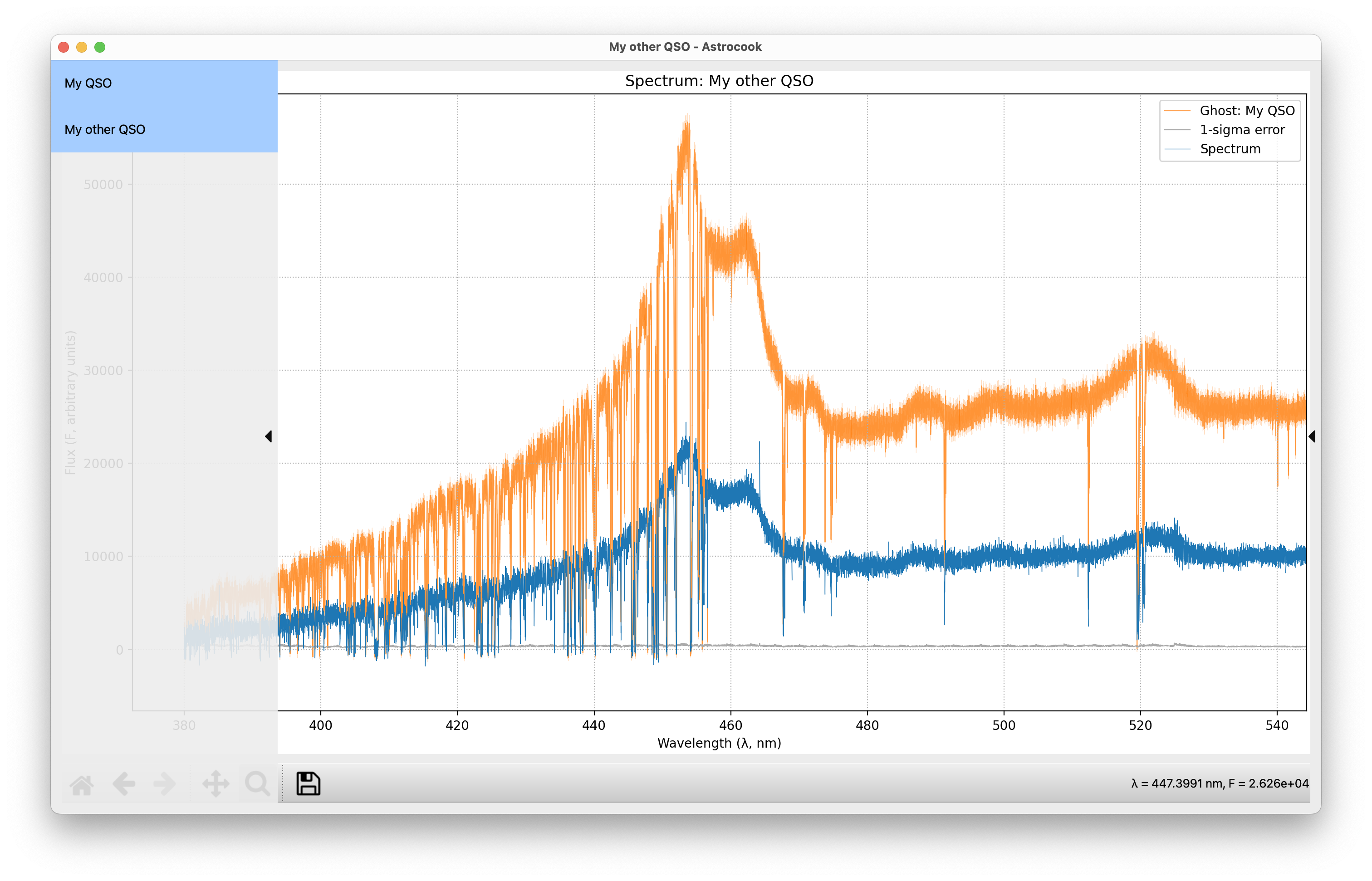
Visualizing Multiple Spectra (Ghost Overlay)#
You can easily compare multiple spectra simultaneously directly in the main plot window:
How to use: Hold
Ctrl(orCmdon macOS) and click on multiple sessions in the left-hand Session List. You can also useShift+Clickto select a continuous range.What you’ll see: Your primary active session remains fully featured (showing models, continuums, and system markers). The additional selected sessions will appear underneath as “ghost” spectra, plotted in distinct, colorblind-friendly colors with semi-transparent flux and error bands. A legend will automatically appear to help you identify them.
Smart Scaling: The ghost spectra are fully integrated with your View Controls! If you toggle Normalize F, all visible spectra will automatically rescale to match the active view.
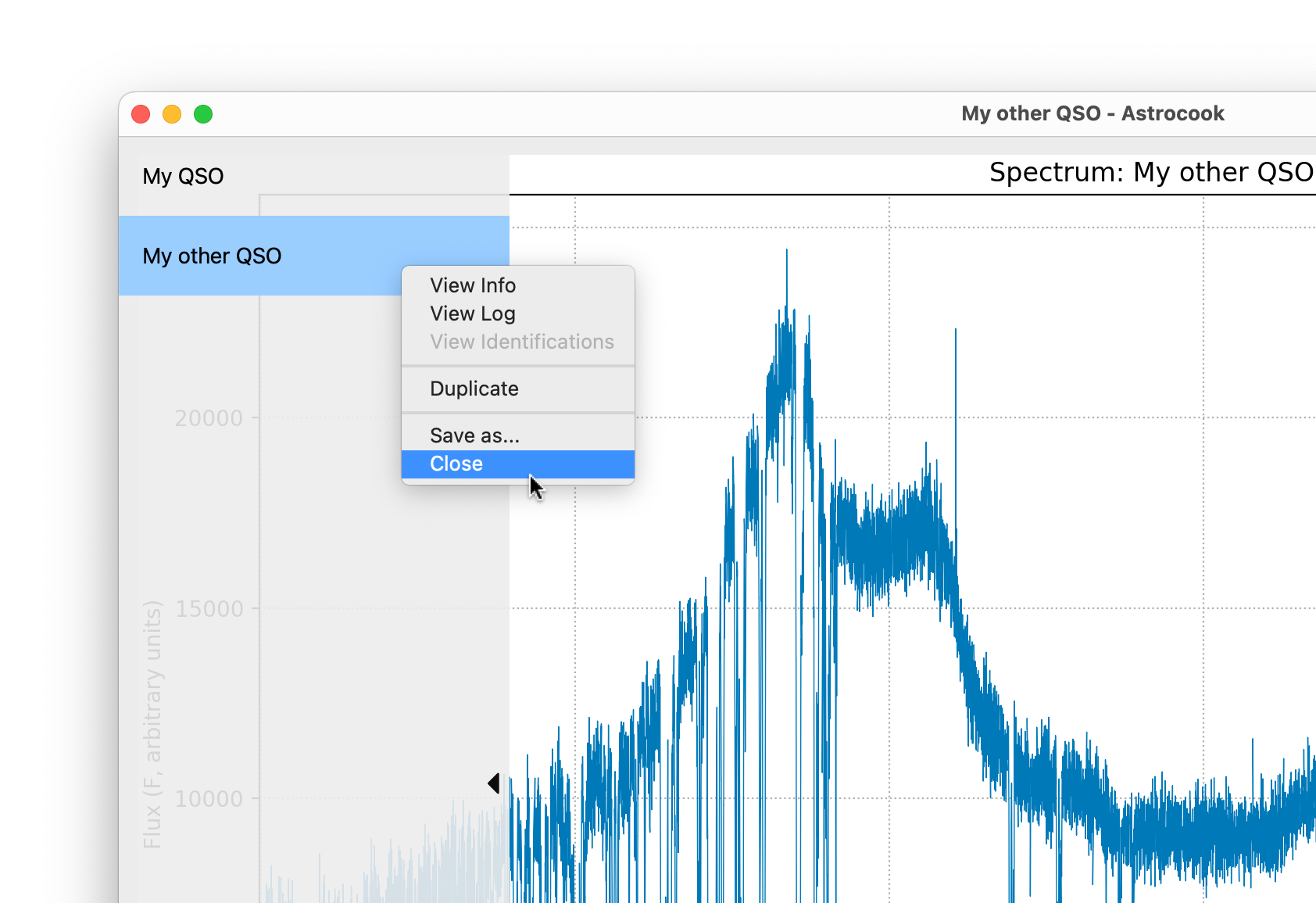
Session Info & Properties#
Right-click on any session in the list to open the context menu. This menu offers several powerful tools:
View Info: Opens the Session Inspector. Here you can see (and edit) critical metadata:
Object Name
Emission Redshift (\(z_\mathrm{em}\)): Crucial for many recipes like the Ly-\(\alpha\) forest analysis.
Resolution (\(R\)): Essential for accurate Voigt profile fitting.
Note
Setting a global resolution here will automatically generate a pixel-by-pixel
resolcolumn across your entire spectrum, which you can verify in the Data Inspector.Duplicate: Creates a complete copy of the current session. This allows you to branch your analysis (e.g., to test two different continuum fits on the same data).
The Log Scripter#
Astrocook automatically records every operation you perform (smoothing, fitting, editing). Right-click a session and select View Log to open the Log Scripter.
This dialog allows you to:
Review History: See a readable list of every recipe run on this session.
Undo/Redo: Step back through your analysis history.
Tip
You can access Undo/Redo also from the Edit menu (see Editing Data) or using the standard key combinations
Ctrl+Z/Ctrl+Y(Cmd+Z/Cmd+Shift+Zon Mac).Run All: Re-run the entire analysis pipeline from the original raw data.
Save Script: Export your workflow as a Python-compatible JSON script for reproducibility.
Saving and Closing#
When you have finished your analysis (or if you want to save your progress):
Save: Go to File > Save Session… or right-click the session in the list. This saves your work as an
.acs2file, preserving all your continuum fits and line lists.Close: You can close a specific session via the right-click menu, or close the active session via File > Close Session.
5. Exporting and Importing Data#
Astrocook allows you to easily exchange data with external tools (like spreadsheet managers, Topcat, or custom Python scripts) using standard CSV files.
Export to ASCII#
To save your current data in a human-readable format, go to File > Export to ASCII…. A dialog will appear allowing you to select exactly what to export:
Spectrum (spec): Saves the Wavelength (\(x\)), Flux (\(y\)), Error (\(dy\)), Continuum (\(cont\)), and any other active spectral columns into a
_spec.csvfile.System List (systems): Saves your identified absorption lines (including Redshift, Column Density, Doppler Parameter, etc.) into a
_systems.csvfile.
You can choose to export entire structures or pick individual columns. The suggested filename will automatically adjust based on your selection, and Astrocook will warn you if you are about to overwrite existing files.
Import from ASCII#
If you have manipulated your exported _spec.csv data externally, you can bring it back into Astrocook by going to File > Import from ASCII….
Astrocook will match the column headers in your CSV to the columns in the active session and overwrite them.
Safety first: The imported file must have the exact same number of rows (pixels) as your current spectrum. Because this operates through the recipe pipeline, the import is fully undoable via the Log Scripter or
Ctrl+Z(Cmd+Z).
What’s Next?#
Now that you are comfortable with the interface, you are ready to manipulate your data. Check out the Editing Data tutorial to learn how to clean up your spectra.